Thinking in: Linear Algebra part 2

Linear algebra is a branch of mathematics that is foundational to machine learning. Mastering it acts as the starting point to seeing data more beautifully.

Welcome to Part 2 of the linear algebra series. In part 1, we discussed scalars, vectors and compared the performance efficiency of NumPy arrays vs Python lists.

In part 2, we will be focusing on vector arithmetic and other operations. After completing this part, you will be to:

• Understand vector arithmetic operations

• Comprehend dot product, eigenvalue, eigenvector and understand their significance in real-world scenarios.

Following are the links to all the parts of the series:

• Part 1 - Scalars, Vectors, NumPy and Python list

• Part 2 - Vector arithmetic and its interpretation

• Part 3 - Advanced Numpy Operations and Optimization

---

Vector Arithmetic

The heart of linear algebra is in two operations-both with vectors.

• We add vectors to get v + w

• We multiply them by numbers c and d to get cv and dw

	import numpy as np
	# Addition of List. This does'nt give the vector addition and instead will concatenate
	z = x + y
	print("x + y is {} and has type {} and is actually concatenation of Elements in the list".format(z,type(z)))
	# Vector addition using Numpy
	z = np.add(x, y)
	print("\nx + y is {} and has type {} and is now add using np.add which results in vector addition".format(z,type(z)))
	# Direct Addition of Array
	c = a+b
	print("\na + b is {} and has type {} and can be directly added as they are arrays".format(c,type(c)))

view raw gistfile1.txt hosted with ❤ by GitHub

Combining those two operations (adding cv to dw) gives the linear combination cv + dw

A few observations

1. Addition of vectors of type: lists using ‘+’ will result in the concatenation of the values

2. Addition of vectors of type: lists using np.add()will result in natural addition of the elements i.e NumPy does the type conversion

3. Addition of vectors of type: ndarry using ‘+’ will result in natural addition of the values

---

The Dot Product

The dot product is an algebraic operation that takes two equal-length sequences of numbers (vectors) and returns a single number.

The dot product is a simple multiplication of each component from both vectors added together

• The result of a dot product between two vectors isn’t another vector but a single value, a scalar

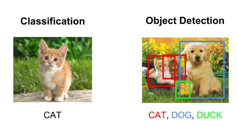
If we have 3 feature vectors. One for each of three images, one of a dog another of a cat, and one unknown; and you would like a machine-learning algorithm to tell you which one of {dog, cat} is the more likely label for the unknown image. If the ‘vector’ of your unknown image is closer in direction to the direction of the ‘dog vector’ it will classify as a dog, otherwise, it will classify as a cat.

Dog vs Cat classification

---

The dot product of a vector with itself

When the vector is v = (1,2,3), the dot product with itself is the length of the vector

v· v = ||v||² = (1*1 + 2*2 + 3*3) =14

If the dot product of two vectors is zero is it means that these two vectors are perpendicular. The angle between them is 90°.

To generalize this the dot product of two vectors is equal to the product of the length of the vectors multiplied by the Cosine angle between them

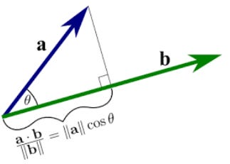
A dot product will tell you how similar in direction vector a is to vector b through the measure of the angle

Let’s execute it with NumPy:

	import numpy as np
	#This is element wise Multiplication
	c = a*b
	print(" * gives elementwise multiplication i.e {} ".format(c))
	# Dot Product
	c=np.dot(a,b)
	print("np.dot gives the dot product of a & b and has value {}".format(c))
	# Interesting thing to notice
	print("\nThe Sum of element wise multiplication will return the dot product i.e sum(a*b) is {}".format(np.sum(a*b)))

view raw gistfile1.txt hosted with ❤ by GitHub

It is a good idea to explore formal definitions of different kinds of vectors (Row vector, Column vector, Unit vector) along with how they are implemented in NumPy and supporting operations. Implementing vectors and visualizing them gives interesting insights and would go a long way into thinking about Linear Algebra.

---

Eigen value and Eigen vector

Eigenvector of a matrix A is a vector represented by a matrix X such that when X is multiplied with matrix A, then the direction of the resultant matrix remains the same as vector X.

Mathematically, the above statement can be represented as:

AX = λX

Here, A is the matrix we are utilizing for analysis and X is the Eigen Vector while λ is the Eigenvalue for the corresponding matrix.

Let us understand through an application of Eigen Vector:

Matrices are of great use while rotating photographs, skewing and creating a mirror image. One feature that you would have surely noticed is that when you warp any photo, one direction remains the same, which is the base of the photo usually. This is the Eigen Vector. An Eigenvector does not change direction while undergoing a transformation.

Eigenvector also helps Google to rank the relevant pages in a jiffy. Goggle forms a “link matrix” which helps to represent the relative importance of each link on a particular topic. This is what makes Google your favourite browser!

Finding Eigenvalue and Eigen vectors is easy in NumPy:

	import numpy as np
	from numpy import linalg as LA
	A=np.array([[1,3],[2,0]])
	λ=LA.eig(A)
	print(λ)

view raw gistfile1.txt hosted with ❤ by GitHub

---

In Part 2, we had a look at some operations on matrices, the dot product, eigenvalues and eigenvectors.

In part 3, we will discuss performance optimization with NumPy.

Following are the links to all the parts of the series:

• Part 1 - Scalars, Vectors, NumPy and Python list

• Part 2 - Vector arithmetic and its interpretation

• Part 3 - Advanced Numpy Operations and Optimization