


Thinking in: Linear Algebra Part 3
Linear algebra is a branch of mathematics that is foundational to machine learning. Mastering it acts as the starting point to seeing data more beautifully.
Welcome to Part 3 in our series on Linear Algebra.
In part 1, we discussed scalars, vectors and compared the performance efficiency of NumPy arrays vs Python lists.
In part 2, we focussed on understanding vector arithmetic operations, comprehending dot product, eigenvalue, eigenvector and understanding their significance in real-world scenarios.
After reading this article, part 3 on linear algebra, you will be able to understand:
Cross product and its significance
Broadcasting and vectorization in NumPy
Performance optimization with NumPy
Following are the links to all the parts of the series:
Part 3 - Advanced Numpy Operations and Optimization
To stay in touch and support us, please subscribe to Coffee and Engineering :
Cross product and its significance
We read about dot product in part 2 of our linear algebra series and we could conclude that:
The dot product is an algebraic operation that takes two equal-length sequences of numbers (vectors) and returns a single number.
In contrast to the dot product, the cross product is an algebraic operation on vectors in three-dimensional space that returns another vector, perpendicular to both the vectors.

While the dot product accounts for the cosine angle, the cross-product accounts for the sine angle.
Cross product signifies the area between the vectors. When vector A is replicated parallelly at the origin and so is vector B, the area of the parallelogram signifies the cross product.

Some properties of the cross product:
It is zero when both vectors are in the same or opposite direction. This means when the angle between two vectors is 0 or 180 degrees, then the area between the vectors, which is signified by the cross product is minimum.
It is maximum when both vectors are perpendicular to each other. This makes the angle 90 degrees.
It is the minimum when the vectors are at an angle of 270 degrees with each other.
To find the direction of the cross product vector, the right-hand thumb rule is used.
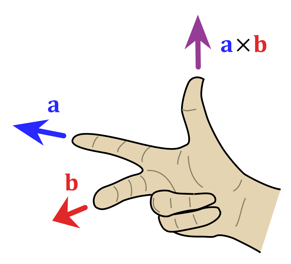
If the index and middle finger denote the vectors A and B, then their cross product vector is represented by the thumb of the right hand.
Cross product can be implemented in NumPy using the following code:
| import numpy as np | |
| # Cross Product | |
| c=np.cross(a,b) | |
| print("np.cross gives the cross product of a & b and has value {}".format(c)) |
Performance Optimization with NumPy
Python is a dynamically typed language which means that you need not declare the variable type while writing the program. The type of variable is checked during the compilation of the program. A program in run line-by-line and compiled into bytecodes, which are then executed. Being dynamically typed, Python is unable to know the variable type in advance.
In other programming languages like C, the variables are declared beforehand and the compiler is aware of it. This enables programmers to optimize the performance in C as they can decide on which variable type can make it faster. Unfortunately, Python does not have this feature and this problem intensifies in loops and nested loops take ages to be executed, as compared to C.
To make the code execution in Python faster, we are left with two options:
Restrict the variable types so that the compilers know beforehand
Eliminate the checking of variable type in every line
Coming to the rescue is NumPy which allows the arrays to have only one data type and stores the data in a block of memory. It uses C at the backend to optimize and speed up the code execution. The functions utilized in NumPy are wrapped on C codes.
Let us try and compare performance of Python loops and Numpy:
| import timeit #importing timeit module to record the time taken in execution | |
| import numpy as np | |
| #creating random list of numbers with a 5x5 matrix | |
| lst1= np.random.randn (5,5) | |
| lst2= np.random.randn (5,5) | |
| #creating a function for multiplication of two arrays using for loop | |
| def multiplication_python (lst1, lst2): | |
| for i in range (len(lst1)): | |
| lst1[i]*lst2 | |
| arr1 = np.array(lst1) | |
| arr2= np.array(lst2) | |
| def multiplication_numpy(arr1,arr2): | |
| arr1*arr2 | |
| #checking the execution time of both functions | |
| %timeit -n 10000 -r 5 multiplication_python(lst1, lst2) | |
| %timeit -n 10000 -r 5 multiplication_numpy(arr1, arr2) | |
The execution of the code above displays the following output:
8.52 µs ± 2.6 µs per loop (mean ± std. dev. of 5 runs, 10000 loops each) 658 ns ± 50.7 ns per loop (mean ± std. dev. of 5 runs, 10000 loops each)The execution time in this particular example shows that NumPy is almost 13 times faster than loop execution in Python!
So we now know that NumPy can make your codes faster but how does it make it possible?
To understand that, we are gonna dive deeper into Vectorization and Broadcasting!
Vectorization
NumPy delegates the loop to a pre-compiled and optimized code in C language. It helps create an Array object which enables to perform operations without involving any loop structures.
The practice of replacing explicit loops with array expressions is commonly referred to as Vectorization. In general, vectorized array operations will often be one or two (or more) orders of magnitude faster than their pure Python equivalents, with the biggest impact in any kind of numerical computations.
— O'Reilly
Apart from the functionality of vectorizing a loop, which performs an operation on two arrays of equal size, we can also vectorize a loop to perform an operation on a scalar and a vector.
One thing to be noticed here is that while using Vectorization, the arrays are of the same size, what can we do when the arrays are not of similar size?
Broadcasting is your friend here!
Broadcasting
The term Broadcasting describes how numpy treats arrays with different shapes during arithmetic operations. Subject to certain constraints, the smaller array is “broadcast” across the larger array so that they have compatible shapes. Broadcasting provides a means of vectorizing array operations so that looping occurs in C instead of Python.
— NumPy
If you will be multiplying two arrays having a dissimilar size, you will be thrown with an error:
operands could not be broadcast together with shapes (3,) (5,5)A set of arrays is called “broadcastable” if one of the following is true:
All the arrays have the same shape
The arrays have the same number of dimension and the length of dimension is either same or 1
The arrays with a low number of dimensions can be made into an array with length 1
Let us understand how to find out if our set of arrays are broadcastable through codes:
| import numpy as np | |
| #creating random list of numbers with unequal shapes | |
| lst1= np.random.randn (1,10) | |
| lst2= np.random.randn (6,10) | |
| lst3= 20 | |
| #Let us check the shapes of all the arrays | |
| lst_arrays = [np.atleast_1d(arr) for arr in (lst1,lst2,lst3)] | |
| for arr in lst_arrays: | |
| print(arr.shape) | |
| def broadcastable (*arrays) -> bool: | |
| try: | |
| np.broadcast (*arrays) | |
| return True | |
| except ValueError: | |
| return False | |
| broadcastable (lst1, lst2, lst3) |
The set of arrays given above satisfy criterion 3, which is why the output of the above code returns a ‘True’ which means that the given set of arrays can be broadcasted.
In Part 3, we had a look at Cross product and its significance, performance optimization with NumPy and understood how performance is optimized in NumPy with Vectorization and Broadcasting.
Following are the links to all the parts of the series:
Part 3 - Advanced Numpy Operations and Optimization
Please share, like and subscribe to Coffee and Engineering!